⚖️ Wheatstone Bridge and Measurement Circuits
The Wheatstone bridge is one of the most elegant measurement circuits ever invented.
Invented in 1833 by Samuel Hunter Christie, popularized by Sir Charles Wheatstone, it's still used today in:
- Strain gauges
- Load cells
- Temperature sensors (RTDs)
- Pressure sensors
- Position sensors
Why? Because it can measure tiny changes with high accuracy.
🔍 What is a Wheatstone Bridge?
A Wheatstone bridge is a diamond-shaped network of four resistors that measures unknown resistance with extreme precision.
The Circuit
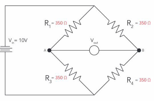
- Four resistors arranged in diamond shape
- R1 (top left) and R2 (top right) form voltage divider from Vex to A
- R3 (bottom left, unknown) and R4 (bottom right) form voltage divider from Vex to B
- Excitation voltage Vex across top and bottom
- Output voltage Vout measured between points A and B (middle nodes)
Nodes:
- Top: Excitation voltage
- Bottom: Ground
- Left middle (A): Between R1 and R3
- Right middle (B): Between R2 and R4
- Output:
📐 The Bridge Equation
Using voltage divider principle:
Output voltage:
⚖️ Balanced Bridge: The Null Condition
When the bridge is balanced:
This occurs when:
Simplifying:
Or:
Solving for unknown :
🎯 Classical Use: Measuring Unknown Resistance
Setup:
- and : Known resistors (ratio arm)
- : Variable precision resistor (standard)
- : Unknown resistor
Procedure:
- Apply excitation voltage
- Adjust until (null detector shows zero)
- Calculate:
Accuracy: Can measure to 0.1% or better!
📊 Example: Measuring 100Ω Resistor
Known values:
- (ratio = 1:1)
- (unknown, approximately 100Ω)
Procedure: Adjust until bridge balances.
Result: at balance
Calculate:
Unknown resistance = 100.2Ω with high precision!
When bridge is balanced, no current flows through the null detector (voltmeter).
This means:
- Voltmeter impedance doesn't matter
- Very sensitive (can detect µV differences)
- Independent of excitation voltage (ratios cancel)
- High accuracy (depends only on resistor ratios)
🏗️ Modern Use: Sensor Interface
Today, Wheatstone bridges are rarely used for null measurement.
Instead, they're used for small changes measurement with sensors:
- Strain gauges
- Pressure sensors
- Load cells
- RTDs (Resistance Temperature Detectors)
🔧 Strain Gauge Measurement
What is a Strain Gauge?
A strain gauge is a resistor that changes resistance when stretched or compressed.
Gauge factor (GF):
Where:
- = fractional change in resistance
- = strain (change in length / original length)
Typical GF = 2 to 2.1 for metallic strain gauges
📏 Strain Gauge Bridge Configuration
Quarter Bridge (1 Active Gauge)
- R1, R2, R4 = fixed resistors (typically 350Ω or 120Ω)
- R3 = strain gauge (changes with strain)
Sensitivity: Lowest (1× gauge output)
Use: Simple, low-cost applications
Half Bridge (2 Active Gauges)
- R1, R2 = fixed resistors
- R3, R4 = strain gauges (opposite strain signs)
Configuration:
- Poisson half-bridge: One gauge in tension, one in transverse direction
- Temperature compensation: Both gauges see same temperature
Sensitivity: 2× quarter bridge
Full Bridge (4 Active Gauges)
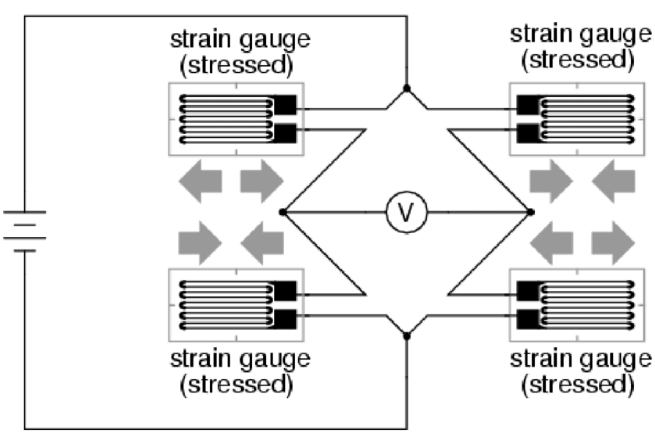
- All four resistors are strain gauges
- Opposite arms experience opposite strains
Configuration:
- R1, R3: Tension
- R2, R4: Compression
Sensitivity: 4× quarter bridge (maximum output!)
Advantages:
- Best temperature compensation
- Highest output
- Common in load cells
⚡ Bridge Output for Small Changes
For small changes in one resistor:
(Quarter bridge, small )
Example: Measuring Strain
Setup:
- Strain gauge: R = 350Ω, GF = 2.1
- Excitation:
- Strain: (1000 microstrain)
Calculate change in resistance:
Bridge output:
Very small signal! Needs amplification (instrumentation amplifier).
🏋️ Load Cell (Weight Measurement)
A load cell is a mechanical structure with strain gauges in full-bridge configuration.

- Aluminum or steel beam
- Four strain gauges bonded to beam
- Top gauges in tension, bottom gauges in compression
- Wired as full Wheatstone bridge
Specifications
Rated output: Typically 2-3 mV/V
Example: 2 mV/V load cell with 10V excitation
- At full load (e.g., 1000 kg): Output =
Sensitivity:
With In-Amp (Gain = 500):
- Full scale:
- Resolution with 12-bit ADC:
🌡️ RTD Temperature Measurement
RTD (Resistance Temperature Detector) is a resistor whose resistance changes with temperature.
Common RTDs:
- Pt100: 100Ω at 0°C, platinum
- Pt1000: 1000Ω at 0°C, platinum
Temperature coefficient:
(For platinum)
RTD in Wheatstone Bridge
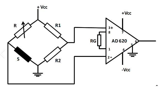
- R1, R2, R4 = fixed resistors (match RTD value at reference temp)
- R3 = RTD (changes with temperature)
Example: Pt100 RTD, measuring 0-100°C
Resistance range:
- At 0°C: 100Ω
- At 100°C:
- Change: 38.5Ω
Bridge output (with ):
At 0°C: Balanced (if R1=R2=R4=100Ω),
At 100°C:
Sensitivity: ~9.6 mV/°C
🛡️ Lead Wire Resistance Compensation
Problem: Long wires to remote sensors add resistance, causing errors.
Solution: Use 3-wire or 4-wire configurations.
3-Wire RTD
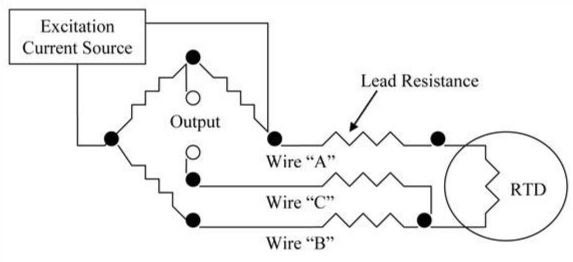
- Third wire added to opposite side of bridge
- Lead resistance appears in both voltage divider arms
- Mostly cancels out (if wires matched)
Result: Reduced error from lead resistance
4-Wire (Kelvin) Connection
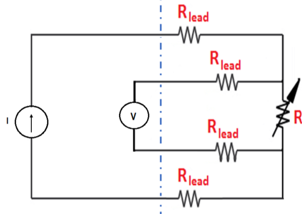
- Two wires for excitation current
- Two separate wires for voltage measurement (high impedance)
- No current in sense wires → no voltage drop!
Result: Zero error from lead resistance!
Used in: Precision measurements, long cable runs
💡 Bridge Excitation: DC vs. AC
DC Excitation
Advantages:
- Simple (just a voltage source)
- Low cost
Disadvantages:
- Thermoelectric voltages (DC offsets)
- Self-heating of sensor
- 1/f noise
AC Excitation
Advantages:
- No DC offsets
- Can use transformers for isolation
- Better noise immunity
- Reduced self-heating (RMS current lower)
Disadvantages:
- More complex (requires demodulation)
- Frequency selection critical
- Phase errors possible
Common frequencies: 400 Hz, 1 kHz, 2.5 kHz, 5 kHz
🎯 Bridge Signal Conditioning
Complete Measurement Chain

- Wheatstone Bridge (sensor)
- Instrumentation Amplifier (INA)
- Low-Pass Filter (anti-aliasing)
- ADC (analog-to-digital converter)
- Microcontroller (data processing)
🔬 Design Example: Weight Scale
Specifications:
- Load cell: 50 kg capacity, 2 mV/V
- Excitation: 10V
- Output range: 0-5V for ADC
- Resolution: 10 grams
Design:
1. Full-scale bridge output:
2. Required gain:
3. Instrumentation amplifier:
Use AD620, set for gain = 250:
Use (1% tolerance)
4. Low-pass filter:
Cutoff frequency = 10 Hz (slow changing weight)
Use
5. ADC:
12-bit ADC (0-5V):
- Resolution:
- Weight resolution:
Meets specification!
🧮 Bridge Nonlinearity
For large changes, bridge output is nonlinear:
Linearization methods:
- Limit range (small changes only)
- Software correction (lookup table or formula)
- Feedback linearization (complex)
For most sensors (strain gauges, RTDs), changes are small enough that linearity error is acceptable.
🛠️ Practical Design Tips
Bridge Design
- Match resistors precisely (0.1% or better)
- Temperature tracking: Use resistors with same TCR
- Excitation stability: Use precision voltage reference
- Shielding: Shield bridge wires from EMI
- Separate ground: Use separate analog ground
Instrumentation Amplifier
- High CMRR: Essential (>100 dB preferred)
- Low noise: Critical for small signals
- Adequate bandwidth: Match sensor response
- Input protection: Clamp overvoltages
Filtering
- Anti-aliasing: Before ADC
- Notch filter: Remove 50/60 Hz if needed
- Digital filtering: In software after ADC
🧪 Lab Exercise: Build a Force Sensor
Objective: Create a force-sensitive button
Components:
- FSR (Force-Sensitive Resistor) or strain gauge
- Three fixed resistors for bridge
- INA128 instrumentation amplifier
- Arduino for ADC and display
Circuit:
- Build quarter-bridge with FSR
- Set bridge excitation = 5V
- Connect to INA128 with gain ~100
- Connect INA128 output to Arduino A0
- Display force reading on serial monitor
Calibration:
- Zero reading (no force)
- Apply known weights
- Create calibration curve
- Implement in software
Challenge: Add temperature compensation!
✅ Key Takeaways
- Wheatstone bridge measures small resistance changes
- Null measurement: Classical method for precision
- Modern use: Sensor interfaces (strain, temperature, pressure)
- Quarter/Half/Full bridge: Trade-offs in sensitivity and compensation
- Instrumentation amplifier essential for small signals
- 4-wire connection: Eliminates lead resistance errors
- Linearization may be needed for large changes
- Complete system: Bridge → INA → Filter → ADC
🎓 Looking Ahead
Bridges are everywhere in measurement:
- Industrial scales and load cells
- Pressure transducers
- Accelerometers (MEMS)
- Torque sensors
- Medical devices (blood pressure, patient monitoring)
Master the bridge, and you can interface almost any resistive sensor!
Next, we'll apply bridges in real applications with amplifiers for load cells and strain gauges!
📚 Further Study
- Experiment with different bridge configurations
- Measure temperature using RTD and bridge
- Build a simple weight scale
- Study impedance bridges (for capacitance/inductance)
- Research AC bridges (for LCR meters)
- Learn about auto-balancing bridges (digital nulling)